Quick intro
Getting familiar with the new tidytext package was a great weekend project. This example follows the structure of the Introduction to tidytext article by the authors of the package, Julia Silge and David Robinson.
The source of the text for this example are tweets. More specifically, tweets with the rstats hashtag. This project will also be an attempt to learn something about the community.
Twitter data import
The twitterR package opens the Twitter API to R users. The config package is used to prevent placing the credentials in the code.
Because these tweets were pulled at a specific point in time, anyone recreating this analysis may get different results.
library(twitteR)token <- config::get()
setup_twitter_oauth(token$key, token$secret, token$token, token$tsecret)## [1] "Using direct authentication"tweets <- searchTwitter("#rstats", 10000)## Warning in doRppAPICall("search/tweets", n, params = params,
## retryOnRateLimit = retryOnRateLimit, : 10000 tweets were requested but the
## API can only return 9050Tidy data
The searchTwitter() function returns a rather complex list object. Using the packages in the tidyverse, the complex list is converted to a tidy table, retweets are removed, and an usable date field is added
library(tidyverse)

tidy_tweets <- tibble(
  screen_name = tweets %>% map_chr(~.x$screenName),
  tweetid = tweets %>% map_chr(~.x$id),
  created_timestamp = seq_len(length(tweets)) %>% map_chr(~as.character(tweets[[.x]]$created)),
  is_retweet = tweets %>% map_chr(~.x$isRetweet),
  text = tweets %>% map_chr(~.x$text)
) %>%
  mutate(created_date = as.Date(created_timestamp)) %>%
  filter(is_retweet == FALSE,
         substr(text, 1,2) != "RT")


tidy_tweets
## # A tibble: 2,389 x 6
## screen_name tweetid created_timestamp is_retweet
## <chr> <chr> <chr> <chr>
## 1 kearneymw 904169552526934017 2017-09-03 02:29:54 FALSE
## 2 ahmad_m_mobin 904167193428074496 2017-09-03 02:20:32 FALSE
## 3 SanghaChick 904166809083027457 2017-09-03 02:19:00 FALSE
## 4 SavranWeb 904165843533213696 2017-09-03 02:15:10 FALSE
## 5 nibrivia 904165791972687872 2017-09-03 02:14:58 FALSE
## 6 Cruz_Julian_ 904162499343376385 2017-09-03 02:01:53 FALSE
## 7 zabormetrics 904157256408813569 2017-09-03 01:41:03 FALSE
## 8 AriLamstein 904156509755637760 2017-09-03 01:38:04 FALSE
## 9 o_gonzales 904151758754238464 2017-09-03 01:19:12 FALSE
## 10 Rbloggers 904149400884215809 2017-09-03 01:09:50 FALSE
## # ... with 2,379 more rows, and 2 more variables: text <chr>,
## # created_date <date>tidytext, transform!
Word tokens
The unnest_tokens() command from the tidytext package easily transforms the existing tidy table with one row (observation) per tweet, to a table with one row (token) per word inside the tweet.
library(tidytext)

tweet_words <- tidy_tweets %>%
  select(tweetid,
         screen_name,
         text,
         created_date) %>%
  unnest_tokens(word, text)

tweet_words
## # A tibble: 37,846 x 4
## tweetid screen_name created_date word
## <chr> <chr> <date> <chr>
## 1 904169552526934017 kearneymw 2017-09-03 new
## 2 904169552526934017 kearneymw 2017-09-03 hex
## 3 904169552526934017 kearneymw 2017-09-03 sticker
## 4 904169552526934017 kearneymw 2017-09-03 for
## 5 904169552526934017 kearneymw 2017-09-03 rtweet
## 6 904169552526934017 kearneymw 2017-09-03 rstats
## 7 904169552526934017 kearneymw 2017-09-03 https
## 8 904169552526934017 kearneymw 2017-09-03 t.co
## 9 904169552526934017 kearneymw 2017-09-03 dfvl8xj2x6
## 10 904167193428074496 ahmad_m_mobin 2017-09-03 pretty
## # ... with 37,836 more rowsStop words
The stop_words table is part of tidytext, it contains common words that can be used to discard from an analysis. This is the kind of list that analysts usually have to find online and then clean up manually.
stop_words ## # A tibble: 1,149 x 2
## word lexicon
## <chr> <chr>
## 1 a SMART
## 2 a's SMART
## 3 able SMART
## 4 about SMART
## 5 above SMART
## 6 according SMART
## 7 accordingly SMART
## 8 across SMART
## 9 actually SMART
## 10 after SMART
## # ... with 1,139 more rowsAn small custom stop words list is put together to reduce the noise caused by terms common in tweets.
my_stop_words <- tibble(
  word = c(
    "https",
    "t.co",
    "rt",
    "amp",
    "rstats",
    "gt"
  ),
  lexicon = "twitter"
)
The combined list of stop words are then used to remove such words from the words in the tweets. An additional filter is added to remove words that are numbers.
all_stop_words <- stop_words %>%
  bind_rows(my_stop_words)

suppressWarnings({
  no_numbers <- tweet_words %>%
    filter(is.na(as.numeric(word)))
})

no_stop_words <- no_numbers %>%
  anti_join(all_stop_words, by = "word")

tibble(
  total_words = nrow(tweet_words),
  after_cleanup = nrow(no_stop_words)
)
## # A tibble: 1 x 2
## total_words after_cleanup
## <int> <int>
## 1 37846 17964More than half of the words in the tweets are considered stop words. Here is a quick look of the words that are currently at the top, based on occurrence:
top_words <- no_stop_words %>%
  group_by(word) %>%
  tally %>%
  arrange(desc(n)) %>%
  head(10)

top_words
## # A tibble: 10 x 2
## word n
## <chr> <int>
## 1 datascience 449
## 2 data 284
## 3 cran 201
## 4 package 196
## 5 machinelearning 108
## 6 rstudio 102
## 7 python 93
## 8 updates 92
## 9 code 88
## 10 y5w2ntksxt 86Sentiment matching
The get_sentiments() functions in tidytext makes it really easy to match words against different lexicons (vocabularies). The NRC lexicon was chosen for this analysis. The get_sentiments() function returns a data frame, a simple table join makes the lexicon part of the analysis.
nrc_words <- no_stop_words %>%
  inner_join(get_sentiments("nrc"), by = "word")

nrc_words
## # A tibble: 4,126 x 5
## tweetid screen_name created_date word sentiment
## <chr> <chr> <date> <chr> <chr>
## 1 904167193428074496 ahmad_m_mobin 2017-09-03 pretty anticipation
## 2 904167193428074496 ahmad_m_mobin 2017-09-03 pretty joy
## 3 904167193428074496 ahmad_m_mobin 2017-09-03 pretty positive
## 4 904167193428074496 ahmad_m_mobin 2017-09-03 pretty trust
## 5 904167193428074496 ahmad_m_mobin 2017-09-03 cool positive
## 6 904166809083027457 SanghaChick 2017-09-03 fun anticipation
## 7 904166809083027457 SanghaChick 2017-09-03 fun joy
## 8 904166809083027457 SanghaChick 2017-09-03 fun positive
## 9 904165843533213696 SavranWeb 2017-09-03 script positive
## 10 904165791972687872 nibrivia 2017-09-03 start anticipation
## # ... with 4,116 more rowsIt is worth mentioning that in the NRC lexicon, one word may have multiple sentiments. For example, the word wait, has a negative and an anticipation classification. From the data joining perspective, this means multiple matches for words that have more than one sentiment.
nrc_words %>%
  group_by(sentiment) %>%
  tally %>%
  arrange(desc(n))
## # A tibble: 10 x 2
## sentiment n
## <chr> <int>
## 1 positive 1225
## 2 trust 770
## 3 anticipation 512
## 4 joy 385
## 5 negative 381
## 6 fear 190
## 7 sadness 180
## 8 disgust 173
## 9 surprise 171
## 10 anger 139Removing that many words from the analysis may mean that there are tweets that had no words that matched NRC. A quick count of the unique tweetid will provide the answer. In this case, all the tweets from tidy_tweets had at least 1 word that matched NRC list.
nrc_words %>%
  group_by(tweetid) %>%
  tally %>%
  ungroup %>%
  count %>%
  pull
## [1] 1362Visualize results
The first visualization is a joyplot using ggplot2 and the new ggjoy extension created by Claus O. Wilke.
library(ggjoy)

  ggplot(nrc_words) +
    geom_joy(aes(
      x = created_date,
      y = sentiment,
      fill = sentiment),
      rel_min_height = 0.01,
      alpha = 0.7,
      scale = 3) +
    theme_joy() +
    labs(title = "Twitter #rstats sentiment analysis",
         x = "Tweet Date",
         y = "Sentiment") +
    scale_fill_discrete(guide=FALSE)
## Picking joint bandwidth of 0.683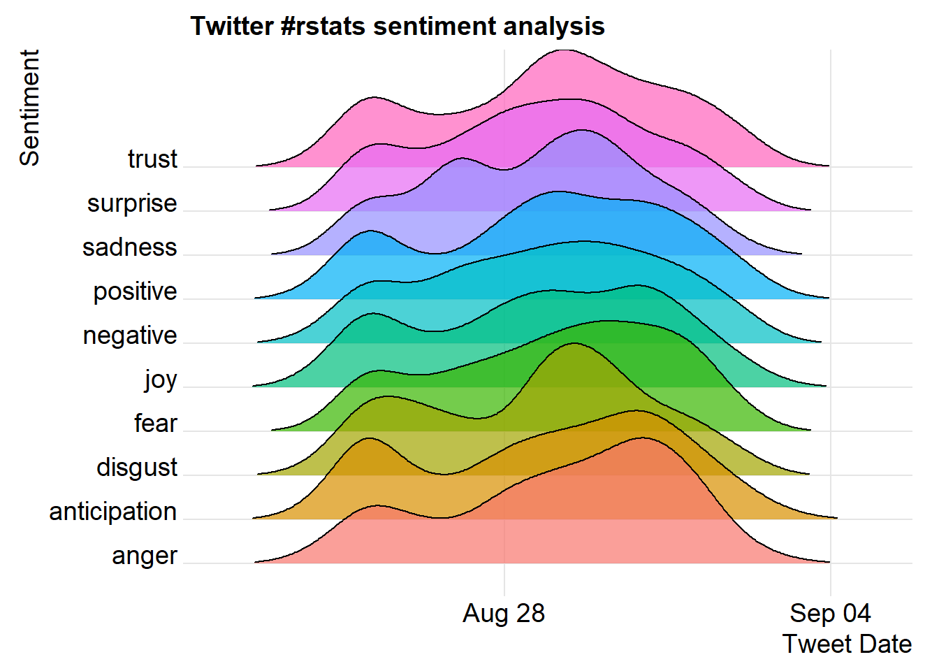
Joyful words
The influence of words classified as “joy” by NRC are analyzed in the wordcloud() function inside the wordcloud package. The words, love and create come out one top.
library(RColorBrewer)
library(wordcloud)


set.seed(10)

joy_words <- nrc_words %>%
  filter(sentiment == "joy") %>%
  group_by(word) %>%
  tally


joy_words %>%
  with(wordcloud(word, n, max.words = 50, colors =  c("#56B4E9", "#E69F00")))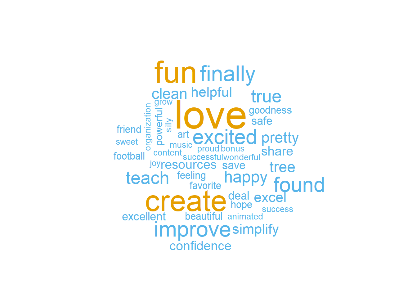
Because a tweet is short, it made sense to find out what words surround joyful words. The next wordcloud will use tweets with at least one word consider joyful. The joyful words are removed, as well as the top 10 orverall words to get a better picture of the surrounding words unique with this sentiment.
other_words <- nrc_words %>%
  filter(sentiment == "joy") %>%
  group_by(tweetid) %>%
  tally %>%
  ungroup() %>%
  inner_join(no_stop_words, by = "tweetid")  %>%
  anti_join(joy_words, by = "word") %>%
  anti_join(top_words, by = "word") %>%
  group_by(word) %>%
  count

other_words %>%
  with(wordcloud(word, nn, max.words = 30, colors =  c( "#56B4E9", "#E69F00")))
## Warning in wordcloud(word, nn, max.words = 30, colors = c("#56B4E9",
## "#E69F00")): proposals could not be fit on page. It will not be plotted.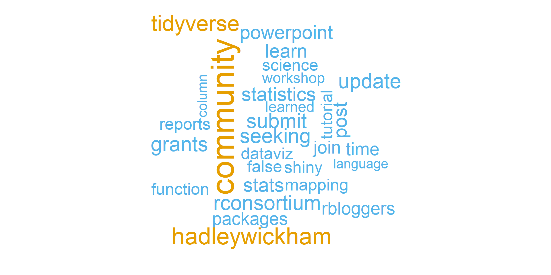
Conclusion
The commentary on the results on the visualizations was limited because I am not a text mining expert. Personally, the results of the “joyful” words was a bit inpirational.
A more objective conclusion is that the tidyverse packages, which seems that it soon will include tidytext, make getting started on text mining easy and actually, fun!